Landscape ecological risk assessment and driving factors in Guyi Basin cultural heritage sites: a multi-scenario simulation perspective

Research framework

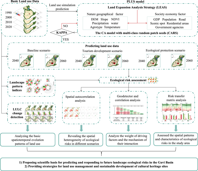
This study systematically evaluates spatiotemporal patterns of LER in China’s Guyi Basin cultural heritage cluster, proposing sustainable protection strategies. First, this study employed the PLUS model to project the spatiotemporal evolution of land use within the Guyi Basin from 2020 to 2060 under three scenarios: baseline, tourism-driven, and ecological protection. Changes in each land-use category were analyzed across space and time. Landscape indices were computed using Fragstats 4.2 to assess the fragmentation, heterogeneity, and connectivity of the Guyi Basin from 1990 to 2060. Subsequently, spatiotemporal patterns of LER in the Guyi Basin for 2020–2060 were evaluated using the LER framework, and spatial autocorrelation analysis was used to reveal spatial heterogeneity in the LER across scenarios. GeoDetector was used to determine the key driving factors and their interactions affecting LER in the study area. This study establishes a framework for assessing LER in the Guyi Basin and provides decision support for sustainable planning at comparable cultural heritage sites (Fig. 1).

Study area

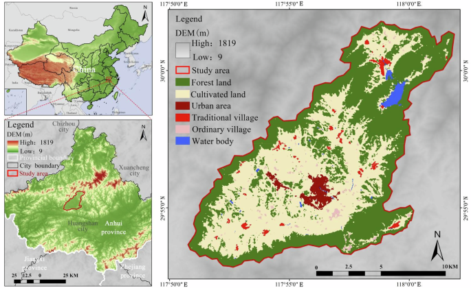
The Guyi Basin lies within the Huangshan Mountains of eastern Anhui Province, China. It also acts as the administrative center of Yi County (Fig. 2). The elevation of the basin varies between 185 m and 679 m, with generally flat terrain. The region enjoys a subtropical monsoon climate, characterized by a humid and warm environment with abundant natural resources, covering about 14755 ha. As the birthplace of Hui culture, the basin is home to 46 nationally recognized traditional villages, forming a unique landscape pattern of settlements, farmlands, and forests. The area’s exceptional cultural legacy and pristine environment have earned it status as a national cultural and ecological protection zone. Compared with 1987, the year when tourism development just started, the annual tourism revenue of Yi County in 2023 reached 14.9 billion yuan, an increase of 1.84 million-fold. In recent years, tourism-driven services have contributed over 50% of the county’s GDP⁴⁰. Nevertheless, the land use structure in the Guyi Basin has been substantially modified due to intense human activity and tourism development, causing decreased land use efficiency and increased ecological risks. The limited ecological carrying capacity, combined with the high intensity of tourism development, makes it a typical region for assessing the equilibrium between socio-economic progress and environmental preservation. This is essential to sustaining effective management of this invaluable heritage site.

Data source and pre-processing

The land-use dataset originated from a publicly accessible national data source, with an overall accuracy of 86.98% ± 0.76%⁴². Four epochs (1990, 2000, 2010, 2020) were analyzed at a 30 m spatial resolution. Based on methodologies from Huang⁴³ and the local environmental characteristics of the study area, four primary land-use categories were distinguished: construction land, forest land, cultivated land, and water body. Additionally, given the complexity of land use types within the cultural heritage site⁴⁴, the “construction land” category was further subdivided. This subdivision was based on field survey records from December 2023, government planning documents, and manual visual interpretation using the ENVI platform. The construction land was divided into Urban area, Traditional village (cultural heritage), and Ordinary village. This classification enables a finer-grained examination of class-specific trajectories under alternative future scenarios (Table 1).

The study incorporates 13 natural-geographical and socio-economic factors in simulating the future land-use structure of the Guyi Basin (Table 2). The future climate, GDP, and population data for 2040 and 2060 are derived from extensively validated public databases. To meet the raster consistency requirements of the PLUS model, a 30 m resolution was applied to all rasters through resampling. For the original 1 km resolution macro-scale data (such as climate), the nearest neighbor method was applied to inherit the parent cell values, reducing the potential introduction of local biases. Bilinear interpolation was applied to high-resolution continuous data factors, such as DEM. The mean difference in factor data before and after resampling was less than 1%. Regarding standard deviation, except for large-scale factors (e.g., temperature), which showed about a 7% variation, the remaining data changes were all below 1%, indicating that the overall error is controllable. Additionally, the study selected eight key factors as driving factors to explore their effects and interactions on LER. These factors include elevation and slope, which reflect terrain constraints; temperature, precipitation, and water systems, which represent ecological resource conditions; scenic areas, which signify tourism pressure; and population and GDP, which indicate the intensity of socio-economic activities. All factors were subjected to multicollinearity testing (VIF < 6). The analysis indicated that redundancy among variables was minimal, except for precipitation and temperature, making them suitable for LER driving factor analysis.

LULC change detection

The land use transition matrix serves as a quantitative methodology designed to characterize conversions among distinct land cover categories, permitting comprehensive evaluation of structural modifications and transition pathways within landscape systems (Eq. (1)).

Where, S signifies the transfer matrix; S_ij defines the spatial extent transitioning from land use type i to j during the study period; n represents the number of landscape types. Implementation typically involves matrix tabulation to decipher patch-type transitions within the Guyi Basin’s landscape configuration.

Landscape pattern indices

Landscape pattern indices serve as effective tools for describing spatial configuration features⁴⁵. Considering the ecological and geographical context of the Guyi Basin and the study objectives, we chose seven representative indices at the landscape and class scales to assess alterations in the composition and configuration of landscapes and land types, focusing on heterogeneity, fragmentation, and connectivity (Table 4). Among these, CONTAG reflects the patch aggregation and clustering degree, while LSI reveals the complexity of land edges, both of which quantify the connectivity and spatial continuity of the landscape; PD, LPI, and AI respectively represent patch density, the proportion of the largest patch, and aggregation trends. All landscape pattern indices were computed with Fragstats 4.2, and their ecological significance is summarized in Table 3.

PLUS model scenario design and validation

In this study, the PLUS model was configured at the patch scale on raster inputs to simulate land use, achieving finer spatial fidelity than integrated models such as MCR, CLUE-S, and FLUS. Distinctively, it incorporates the Random Forest algorithm to investigate land use drivers, achieving superior interpretability and predictive accuracy³⁸. This model synergistically integrates dual methodological approaches. Based on the actual conditions of the Guyi Basin and available data, this study employs 13 factors to simulate and forecast its future land use structure. Land use expansion areas from the 2000 and 2010 datasets were extracted, and the development probability for each land-use class was learned using a Random-Forest classifier. Subsequently, the 2020 land-use pattern was obtained through a cellular automaton employing random patch seeding across classes. The simulation results for 2020 were evaluated using the confusion Matrix and FOM tools (including Kappa and FOM statistical tools), confirming that the model has high simulation accuracy (OA = 0.89, Kappa = 0.82 > 0.8, and FOM = 0.53), and accurately reflect land use pattern changes under future scenarios.

Using the 2000 and 2020 land-use data together with scenario-specific drivers, this study simulates the land-use patterns of the Guyi Basin in 2040 and 2060 under three scenarios: baseline (BS), tourism development (TDS), and ecological protection (EPS). The scenario settings are as follows: the BS continues the historical change trends from 2000 to 2020; the TDS assumes that traditional villages and urban construction will be further strengthened, with an increase in construction land and no land conversion out of construction use; in the EPS, forest and water resources are prioritized, with ecological land conversions to cultivated or construction land constrained. The neighborhood weights and conversion cost matrices for each scenario are defined based on scenario constraints and previous research⁴⁶ and are quantified in Table 4. Conversion restrictions among land types are represented using a land use conversion matrix, with 0 denoting prohibited conversions and 1 denoting permissible ones; the neighborhood weights range from 0 to 1, where a larger value indicates stronger expansion intensity and neighborhood influence for that land type. To assess the robustness of PLUS model predictions, a sensitivity test was conducted for the 2060 BS by perturbing neighborhood transition weights of each land use type by ±10% and resimulating the land use patterns³⁸. The results showed minimal changes compared with the baseline simulation for 2060 (OA = 0.915 > 0.90, Kappa = 0.85 > 0.80).

Landscape ecological risk assessment

According to previous studies, differences in LER among zones are shaped by both land-use structure and its spatial configuration. We employed a landscape-pattern-based approach⁴⁷ and developed a comprehensive LER evaluation model by integrating landscape loss (LLI), vulnerability (LVI), and disturbance index (LDI) to assess and quantify LER values in the study area²⁵.

This study employs an equidistant grid sampling method. Guided by the spatial configuration of land use patches (size distribution and dispersion patterns), the study area was partitioned into 679 analytical units of 0.5 km × 0.5 km resolution using ArcMap 10.8. Building upon the PLUS-model-simulated LER spatial distributions for 2020 and 2060 under three development scenarios, grid-level ERI values were derived from the central point ERI of each ecological risk unit, and Kriging interpolation was employed to generate the spatial distribution of LER across the study region⁴⁸. Drawing on the study area’s features and prior research²⁵, the Jenks natural breaks method was applied to divide LER into five classes, from lowest to highest. External validation with Normalized Difference Vegetation Index (NDVI) and Normalized Difference Water Index (NDWI) at the 0.5 km grid (n = 679) showed coherent gradients across levels (Kruskal–Wallis: NDVI H = 193.226 > 0; NDWI H = 294.163 > 0; both p < 0.001) and correlations with the risk rank (NDVI r = −0.574; NDWI r = 0.672; both p < 0.001), supporting the ecological rationale of the classification. Finally, this study computes a composite LER metric by integrating the LLI, LVI, and LDI.

First, the LER index represents the relative value of ecological loss in the study area due to external influences, calculated with Eq. (2).

Where ERI_i indicates the ecological risk index of the i-th risk unit; within the k-th zone, A_ki refers to the area of land-use type i, and A_k denotes the total area of the k-th risk zone.

Second, the LLI measures ecological damage across landscape types under external pressures by combining the LDI and LVI. The LVI, derived from expert elicitation and normalized, is assigned as follows: cultivated land (0.190), forest land (0.095), water bodies (0.143), urban construction land (0.238), ordinary rural land (0.048), and cultural heritage land (0.286). (Eq. (3)).

Finally, the LDI evaluates how external disturbances affect various landscape types in the natural ecosystem (Eq. (4)).

Where C_i, S_i, and D_i represent the normalized fragmentation, separation, and dominance indices, respectively. The weights a, b, and c were set to 0.5, 0.3, and 0.2, informed by the study-area context and relevant literature.

Spatial autocorrelation analysis

As a fundamental technique in spatial statistics, spatial autocorrelation analysis encompasses a suite of techniques, including both global and local measures. Global autocorrelation captures the overall clustering or dispersion of LER across the study area, quantified by Moran’s I (–1 < I < 1; Eq. 9). A value close to 1 reflects pronounced spatial positive/clustering, whereas a value near −1 denotes negative/dispersion in the study object (Eq. (9)). Statistical significance is assessed via a Z-score, with |Z | > 1.96 denoting significant spatial autocorrelation.

Local spatial characteristics were assessed using Local Moran’s I, a statistic of local spatial autocorrelation. This analysis captures the tendency towards spatial clustering (homogeneity) or dispersion (heterogeneity) of the target variable across its geographical locations⁴⁹. The outcomes are categorized into four distinct spatial patterns: High-High (HH), High-Low (HL), Low-High (LH), and Low–Low (LL), as derived from Eq. (10).

Where n denotes the total number of spatial units; x_i and x_j refer to the LER values at units i and j; the mean LER of the study area is expressed as \(\overline{x}\); and w_ij represents the spatial adjacency between the two units, taking 1 for adjacent and 0 for non-adjacent pairs.

Geodetector analysis

GeoDetector is a statistical method used to detect spatial heterogeneity and attribute it to underlying drivers (Eq. (11)). In this study, it is applied to quantify the weight of each driving factor on LER and to evaluate their interactive effects⁴⁹.

The stratification (h = 1, 2, …, L) expresses the heterogeneity of the dependent variable Y (LER) and explanatory factors X. N_h and N indicate the number of units in stratum h and in the entire area, while σh² and σ correspond to their respective variances. The statistic q(0–1) quantifies driver influence, with higher values indicating a stronger effect on LER. The p-value tests significance, where p < 0.05 denotes a significant effect on LER. Interactive analysis assesses whether combinations of factors increase or decrease the explanatory power for Y, classifying interactions into five types. For example, nonlinear enhancement occurs when q(X₁ ∩ X₂) > q (X₁) + q (X₂), indicating synergistic interaction beyond independence.