Sustainable tourism at nature-based cultural heritage sites: visitor density and its influencing factors

Spatial distribution of NCHS and its influencing factors

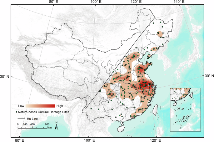
The kernel density analysis results, illustrated in Fig. 1, reveal a pronounced spatial clustering pattern in the distribution of NCHS across China. High-density clusters are observed primarily in the southeastern coastal regions and certain areas of central and western China, particularly the Yangtze River Delta, Pearl River Delta, and Beijing-Tianjin-Hebei regions. These areas are not only economically prosperous but also serve as key regions for the preservation and development of cultural heritage. Additionally, regions in central and western China with a concentration of historical sites, such as Sichuan, Shaanxi, and Yunnan provinces, also exhibit high kernel density values.

Spatial distribution of 238 NCHS.

The results of the OPGD analysis (Table 3) reveal that multiple factors significantly influence the spatial distribution of NCHS. Among the 13 analyzed variables, cultural institutions, education, religion and folklore, GDP per capita, historical settlements, road density, temperature, and FVC all passed the 5% significance level test, indicating that cultural, economic and environmental factors contribute to the spatial pattern of NCHS. Cultural institutions and education exert the strongest influence, highlighting the pivotal role of cultural and educational resources (q > 0.2). Social-economic factors, including GDP per capita and road density, have a moderate impact (0.1 < q ≤ 0.2), suggesting that economic development and accessibility contribute significantly to the distribution of these sites. Religion and folklore, historical settlements, temperature and FVC also exert notable effects, though to a lesser extent (0.05 < q ≤ 0.1). In contrast, factors such as elevation, topographic relief, river density, precipitation, and population density do not show significant effects. These findings indicate that while natural environmental conditions may influence the spatial distribution of NCHS, their impact is relatively limited compared to cultural, economic, and infrastructural variables.

Spatial distribution of visitor density in NCHS

The visitor density analysis, presented in Fig. 2, highlights distinct spatial heterogeneity in the distribution of visitor density across NCHS. This variability is likely influenced by factors such as the cultural heritage value of the sites, transportation accessibility, natural landscape characteristics, and the level of tourism development. Visitor density is notably higher in the southeastern coastal areas and northwestern regions of China, with hotspots in the Yangtze River Delta, the west coast of the Taiwan Strait, and Shaanxi Province. These findings suggest that these regions possess significant cultural heritage value and strong tourism appeal. Conversely, lower visitor density is observed in central and remote western regions, likely due to limited transportation infrastructure and relatively underdeveloped tourism. Interestingly, the results of the kernel density analysis and visitor density analysis demonstrate similar spatial distribution patterns, particularly in the pronounced visitor clustering observed in southeastern coastal regions such as the Yangtze River Delta.

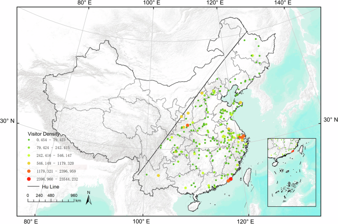
Spatial distribution of visitor density of 238 NCHS.

Correlation analysis and OLS model

Figure 3 presents a heatmap of the Spearman correlation coefficients between all landscape variables and visitor density for NCHS. The results reveal that the strongest and most significant correlation is between visitor density and Den_CH (β = 0.81, p < 0.001), indicating that areas with higher cultural heritage density attract more visitors. This finding aligns with the understanding that cultural heritage sites tend to draw larger numbers of visitors, particularly in areas with concentrated cultural significance. Additionally, visitor density is positively correlated with Den_road, Den_museum, and Den_SF. In contrast, it shows a negative correlation with natural landscape indicators such as FVC and elevation. These correlations suggest that while infrastructure and cultural facilities contribute to higher visitor density, natural landscape features like vegetation cover and elevation may have an inhibitory effect on visitor concentration. Spearman correlation analysis measures the monotonic relationship between two variables but does not imply causation. In contrast, regression analysis establishes a linear relationship between a dependent variable (Y) and one or more independent variables (X), allowing for prediction and causal inference. The subsequent regression analysis will further explore the combined effects of these indicators on visitor density.

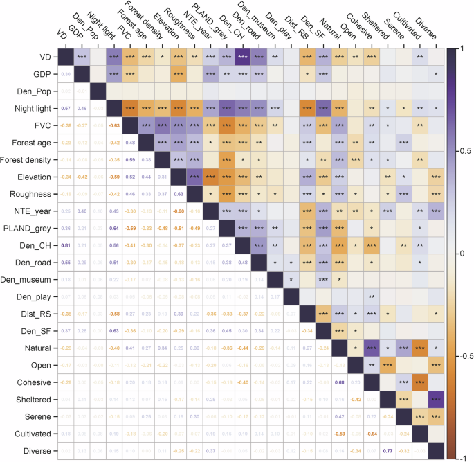
*p < 0.05, **p < 0.01, ***p < 0.001; The numbers in the squares of the figure are Spearman’s rank correlation coefficients.

To evaluate the relative contributions and effects of natural variables, artificial variables, and perception variables on visitor density, this study established a baseline model (Model 0) incorporating only covariates. Subsequently, three additional models were constructed by adding natural variables (Model 1), artificial variables (Model 2), and perception variables (Model 3) to the baseline model. Finally, all variables across the three dimensions, along with covariates, were integrated into a comprehensive model (Model 4) to assess the combined multidimensional effects (Table 4). The specifications of the OLS models are as follows:

Model 0: Dependent variables (Y) ∼ Covariates

Model 1: Dependent variables (Y) ∼ Covariates + Natural variables

Model 2: Dependent variables (Y) ∼ Covariates + Artificial variables

Model 3: Dependent variables (Y) ∼ Covariates + Perception variables

Model 4: Dependent variables (Y) ∼ Covariates + Natural variables + Artificial variables + Perception variables

Table 5 presents the results of the five OLS models. The baseline model (Model 0) explains 6% of the variance in visitor density, whereas the comprehensive model (Model 4) explains 52.4%. The Variance Inflation Factor (VIF) values for all models are below 10, indicating that multicollinearity is not an issue in the models.

The improvement in model performance, measured by the adjusted R², highlights the contribution of each dimension of variables to visitor density. Compared to the baseline model (R² = 0.060), Model 1 (R² = 0.369), Model 2 (R² = 0.387), and Model 3 (R² = 0.092) demonstrate increases of 0.309, 0.327, and 0.032, respectively. These results indicate that artificial variables have the greatest impact on visitor density, followed by natural variables, while perception variables have the least influence. The comprehensive model (Model 4) achieves the best fit (R² = 0.524), with improvements of 0.155, 0.137, and 0.432 compared to Models 1, 2, and 3, respectively.

The regression results of Model 4 identify 10 variables with significant effects on visitor density. Among these, four variables exhibit negative impacts: FVC (β = –0.254, P < 0.01), NET_year (β = -0.254, P < 0.01), Den_road (β = -0.254, P < 0.01), and Den_SF (β = –0.254, P < 0.01). The remaining six variables demonstrate positive effects. The three variables with the strongest contributions are NET_year (β = –0.254, P < 0.01), Den_CH (β = 0.300, P < 0.01), and PLAND_grey (β = 0.257, P < 0.001).

Spatial autocorrelation analysis and spatial regression models

This study conducted an LM test on Model 4 (Table 6), yielding a Moran’s I value of 3.5171 (P < 0.01), indicating significant spatial autocorrelation in the OLS residuals. The presence of notable spatial dependence suggests that the OLS model may be insufficient to capture the spatial structure of the data, necessitating further analysis using spatial regression models. The significant result of the Lagrange Multiplier (error) test (P < 0.05) suggests that SEM is more appropriate for addressing spatial effects, thereby ensuring more reliable estimation results. To compare the performance of spatial models, the study examined the results of the OLS model (Model 4), SEM (Model 5), and SLM (Model 6).

Table 7 presents the results of the spatial regression models for visitor density. Model selection was based on information criteria, including the Akaike Information Criterion (AIC) and Schwarz Criterion (SC), where smaller values indicate better model fit. The OLS model had an adjusted R² of 0.524. When spatial effects were incorporated, the SEM demonstrated an improvement in R² compared to the OLS model, whereas the SLM did not show changes in R². Additionally, the SEM exhibited the lowest AIC and SC values among the three models. Based on these findings, SEM (Model 6) was selected as the final spatial regression model for analyzing the relationship between landscape characteristics and visitor density in NCHS.

The results of the SEM are summarized in Table 7. LAMBDA, representing the spatial error coefficient (λ) in the SEM equation, was found to be significant at the 0.001 level, confirming the presence of significant spatial dependence. A total of 10 variables were identified as having a significant influence on visitor density. Five variables exhibited a significant positive correlation with visitor density: GDP (P < 0.05), forest age (P < 0.01), PLAND_grey (P < 0.001), Den_CH (P < 0.001), and “Natural” perception (P < 0.01). Conversely, five variables demonstrated a significant negative correlation with visitor density: FVC (P < 0.001), NET_year (P < 0.001), Den_road (P < 0.001), Den_SF (P < 0.01), and “Cohesive” perception (P < 0.05).

Relative importance analysis of XGBoost-SHAP

The dataset was divided into a training set and a test set in a 7:3 ratio. Hyperparameters were optimized using the grid search method^54,55, and the optimal XGBoost model parameters were determined through K-fold cross-validation, where K = 5 in this study. The model’s performance was evaluated based on the root mean square error (RMSE)^56,57. The final optimal parameter combination identified was as follows: learning_rate = 0.01, max_depth = 5, and n_estimators = 100, yielding a minimum RMSE of 1834.4. The final model trained with these parameters served as the basis for calculating SHAP values. To identify the key factors influencing visitor density in NCHS, the absolute SHAP values (mean|SHAP | ) were used. SHAP analysis revealed the contribution of natural variables, artificial variables, and perception variables to visitor density based on Shapley values. A higher SHAP value indicates a greater influence of a variable on the model’s predictions.

Figure 4a presents the results of global feature importance. The findings highlight that FVC and Den_CH have the greatest influence on visitor density, with most artificial landscape indicators ranking prominently. Figure 4b illustrates the results of local feature importance, where each data point represents an NCHS. The color of each point reflects the feature value, with red indicating high values and blue indicating low values. The x-axis represents SHAP values, which can be either positive or negative, signifying both the magnitude and direction of a variable’s impact on the model’s output.

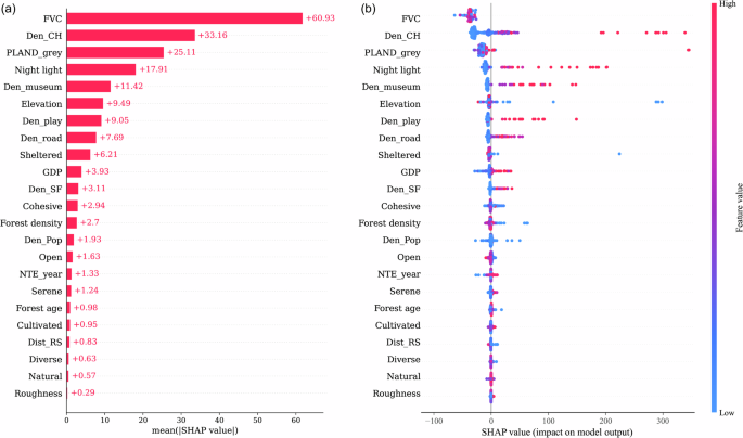
a Global feature importance. b Local feature importance.

The results presented in Fig. 5 further illustrate the impact of different landscape dimensions on visitor density. Collectively, natural landscapes contribute 37.11% to visitor density, artificial landscapes account for 44.30%, and landscape perception contributes 6.94%. These findings indicate that artificial landscapes exert the greatest influence on visitor density, followed by natural landscapes, while the effect of landscape perception is relatively minimal.

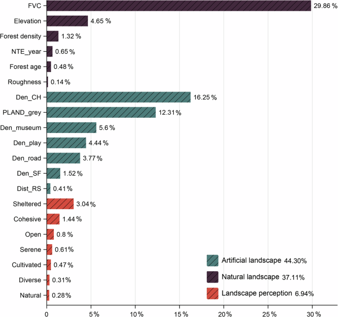
Contribution of variables in the three dimensions.

Within each dimension, individual indicators show varying levels of influence. Among natural landscape indicators, FVC is the most impactful, with a contribution rate of 29.86%, followed by elevation at 4.65%. The effects of other natural indicators are relatively minor. In the artificial landscape dimension, Den_CH has the highest influence, contributing 16.25%, followed by the proportion of gray spaces and museums, with contribution rates of 12.31% and 10.56%, respectively. In the perception dimension, most indicators exhibit relatively low importance. However, the “Sheltered” and “Cohesive” dimensions show comparatively greater influence, with contribution rates of 3.04% and 1.44%, respectively. Other perception indicators have a negligible impact on visitor density.

Interactions and threshold effects of XGBoost-SHAP

The partial dependence plots (PDPs) in Fig. 7 provide a deeper understanding of the interaction effects between cultural heritage density (Den_CH) and other variables across three dimensions—natural variables (FVC), artificial variables (Den_museum), and perception variables (Cohesive). The analysis also reveals the threshold effects of cultural heritage density on visitor density. In the plots, the x-axis represents the actual values of Den_CH, while the y-axis corresponds to its SHAP values, indicating the contribution of Den_CH to the model predictions. The data points are color-coded to reflect the values of the interacting features, with blue denoting lower values and red indicating higher values.

In regions with higher cultural heritage density, lower vegetation coverage is often associated with higher visitor density (Fig. 6a). This suggests that cultural heritage characteristics may attract more visitors even in areas with less abundant vegetation. A plausible explanation is that the cultural significance of these heritage sites serves as the primary draw for visitors, with vegetation playing a secondary role. Additionally, areas with lower vegetation coverage may feature more open spaces or better accessibility, further contributing to increased visitor flows. Regions with higher cultural heritage density and the presence of multiple museums tend to attract more visitors (Fig. 6b). This indicates that in areas rich in cultural heritage, the presence of museums enhances regional appeal and drives higher visitor density. Museums, as part of the cultural landscape, provide educational value, historical context, and immersive experiences, enhancing the attractiveness of the destination and contributing to a richer tourism experience^58,59,60. In areas with lower spatial cohesion, higher cultural heritage density is associated with increased visitor density (Fig. 6c). This suggests that dispersed spaces, such as heritage sites divided by walls or steps, tend to attract more visitors. The dispersed layout may create additional points of interest, encouraging visitors to explore various parts of the site, thereby enhancing their overall experience. Conversely, higher spatial cohesion might result in a more unified site layout, which may reduce visitors’ inclination to explore beyond the main attractions.

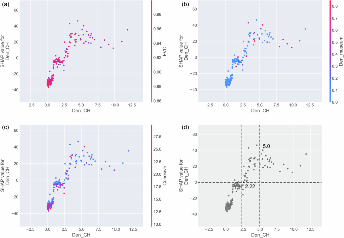
a Interaction effect between Den_CH and FVC. b Interaction effect between Den_CH and Den_museum. c Interaction effect between Den_CH and Cohesive perception. d Nonlinear relationship and threshold effects of Den_CH on visitor density.

The relationship between visitor density and cultural heritage density is nonlinear (Fig. 6d), with two critical threshold points: the first at 2.22, where the relationship shifts from negative to positive, and the second at 5.0, representing a saturation peak. This indicates that as cultural heritage density increases, there is a critical point (2.22) where its impact on visitor density becomes positive. Beyond this point, visitor density continues to rise until it peaks at 5.0, after which growth begins to stabilize or decline. These thresholds highlight the nonlinear dynamics between cultural heritage density and visitor attraction.

Interaction detection of OPGD

The results obtained from the optimal-parameter geographical detector comprehensively illustrate the interactive effects among influencing factors on visitor density across China’s NCHS, highlighting varying interaction intensities and distinct interaction types (Fig. 7). According to the analysis, the interactions among these influencing factors predominantly exhibit nonlinear enhancement and bivariate enhancement effects, suggesting that the combined influences of these factors substantially exceed the sum of their individual impacts. Specifically, socioeconomic factors show pronounced nonlinear enhancement interactions with natural landscape variables (e.g., Forest density and Roughness), artificial landscape variables (e.g., Den_road and Dist_RS), and visitor-perception variables (e.g., Natural, Open, Cohesive, and Cultivated). Among natural landscape variables, significant interactions are observed between Forest density and Elevation, as well as between Roughness and NTE_year, indicating strong synergistic relationships affecting visitor density.

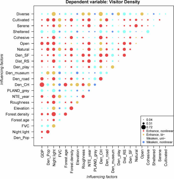
The interactive effects of influencing factors on the visitor density of NCHS.

Within artificial landscape factors, the interaction between cultural heritage density (Den_CH) and GDP exerts the strongest influence on visitor density, with an interaction q-statistic reaching as high as 0.7213. This finding suggests that the combined effect of socioeconomic status and cultural heritage density significantly enhances site attractiveness. Moreover, substantial interactive effects are observed between Den_CH and other variables such as Forest age, Den_road, Dist_RS, Cohesive, and Den_SF. Conversely, the interaction between Den_CH and vegetation coverage (FVC) is relatively weak, which aligns well with previous findings obtained from the XGBoost-SHAP model analysis. Regarding visitor-perceived factors, the nonlinear enhancement interaction between Natural and Serene demonstrates the highest magnitude, underscoring their combined importance in influencing visitor preferences. Interestingly, variables such as PLAND_grey and Sheltered consistently exhibit weak interaction types with all other factors. Collectively, these findings elucidate the complex interplay among socioeconomic, natural landscape, artificial landscape, and visitor-perceived factors in shaping visitor density patterns at China’s NCHS, providing valuable insights for future planning and sustainable tourism management.